H2020 Project: Sensor Fusion Calibration for Low-Cost Air Quality Monitoring
This blog post explores the calibration of low-cost sensors for urban air quality monitoring through sensor fusion strategies, focusing on a subset of data across Europe. It evaluates various calibration models to enhance sensor accuracy and reliability in measuring ozone concentration, highlighting the potential for cost-effective, dense monitoring networks.
Analysis Goal
Urban air quality monitoring requires a dense network of monitoring stations to effectively map out the distribution of air quality across regions. However, due to the high cost of certified analyzers, the density of monitoring stations has been low. Low-cost sensors have been proposed as a solution to this challenge because they are inexpensive to deploy and can be calibrated by a certified analyzer for a short time before being used in the field for an extended period.
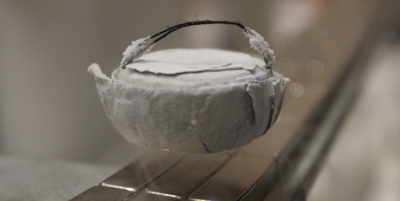
This dataset contains raw data from 25 sensor nodes distributed across Austria, Spain, and Italy, with six sensors within each node: four metal oxide sensors, one temperature sensor, and one relative humidity sensor. The metal oxide sensors contained in each node are specialized for O3 monitoring. All nodes are first calibrated at a home station in Spain and then recalibrated at a reference station near the target area, followed by field deployment for several months and another recalibration at the reference station.

In this analysis, we will examine the viability of the strategy of using low-cost sensors for high-density air monitoring, as metal oxide sensors tend to drift and age after long-term deployment. Moreover, when the environmental conditions change, they will need recalibration. Since this dataset contains data from multiple locations that require separate treatment, we will look at only a subset of it from one location to test our idea. We will do the following:
- Data loading: The original paper contains only the signals from sensors, and we need to find the reference O3 concentration from external sources.
- Data cleaning: This dataset and reference data contain a lot of missing values, so several rounds of cleaning are required.
- EDA using a correlation matrix and a scattering matrix.
- Calibration models: We will use linear models like multiple linear regression and Lasso regression, and nonlinear models like support vector regressor and random forest regressor to perform the calibration.
- Within each modeling trial, we will investigate the idea of sensor fusion, that is, using more than one sensor within the same node to infer O3 concentration for better robustness to sensor drift and failure.
- In evaluating the performance of calibration algorithms, a series of metrics will be used, including r2 score, RMSE, CRMSE, mean bias error, etc., to examine the bias and variability of the calibration.
- As the sensors are moved between reference stations and calibrated separately, the calibration performance in different locations is also examined.
The full analysis with code can be found in this Kaggle notebook.
Analysis Target Selection
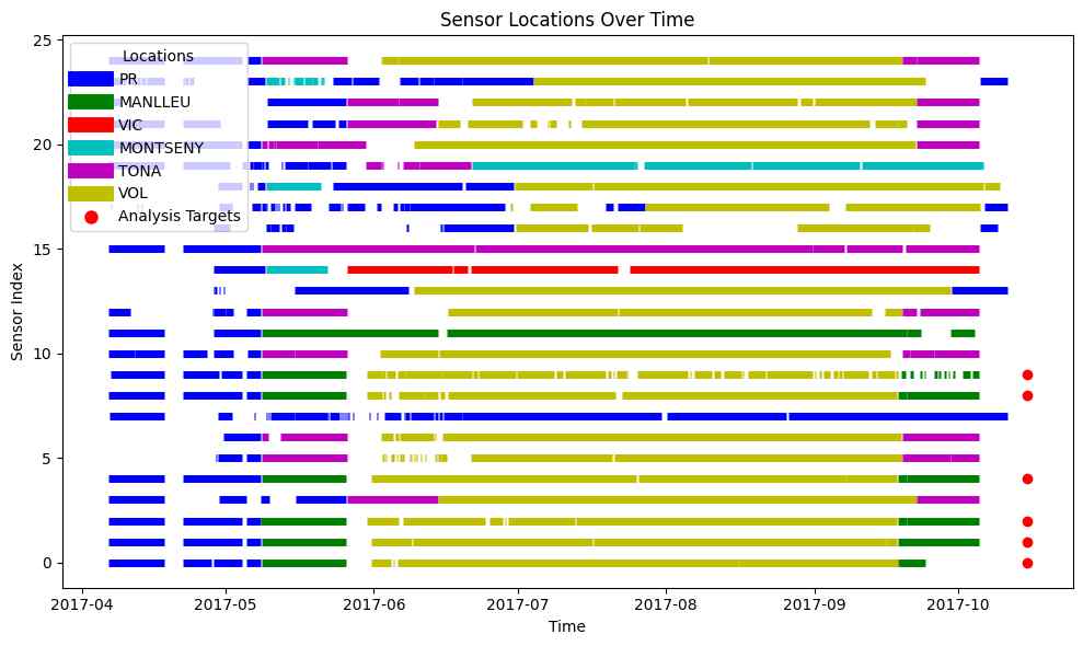
According to the dataset descriptions, the 25 sensor nodes are moved to different locations at different points in time. To control variables, we will select nodes that follow the route of PR -> MANLLEU -> VOL -> MANLLEU as there are six of them in the dataset and their time axis is relatively aligned.
An overview of the sensor node trajectory is presented below, with red dots at the end marking our sensor nodes of interest.
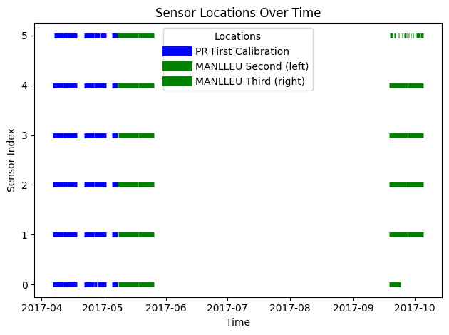
Sensors of Interest
Here we show the six sensor nodes on which we will base our analysis. The time and locations are controlled, making them a natural set of data to perform analysis on. The big time gap between the two MANLLEU periods is the ‘VOL’ periods that have been removed due to the lack of reference data.
EDA
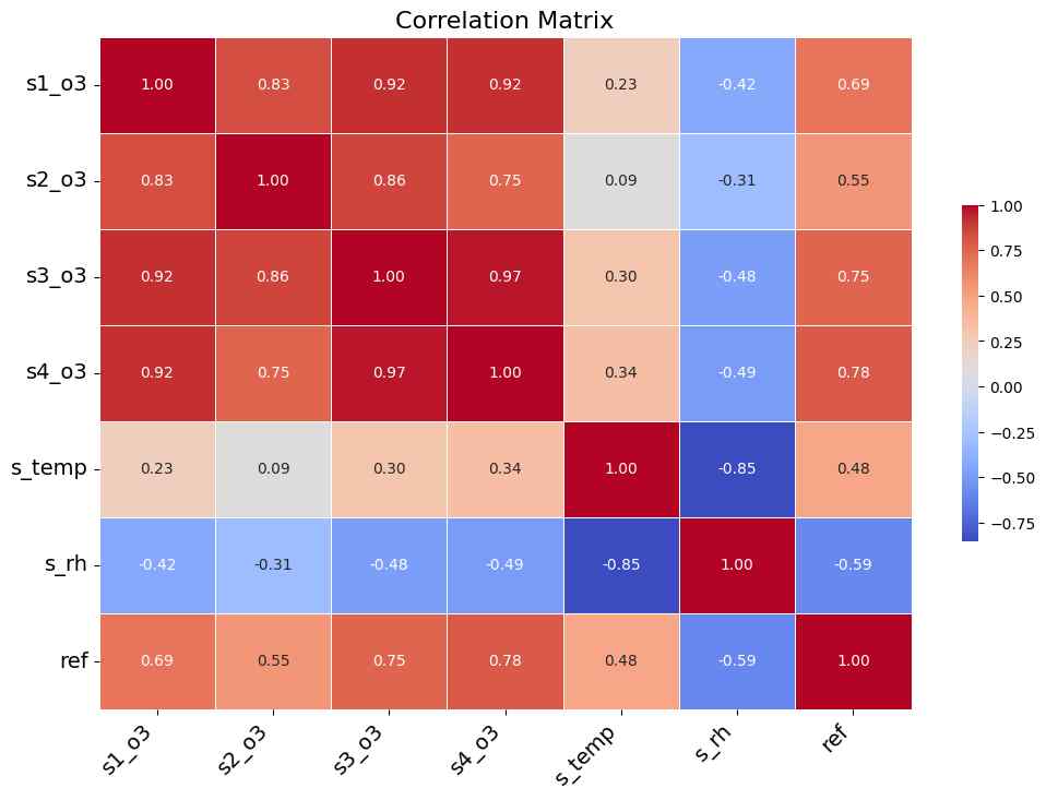
Each sensor node contains six sensors: four low-cost metal oxide sensors, one temperature sensor, and one relative humidity sensor. With true O3 concentration from the reference station appended to the corresponding dataframe, an example correlation matrix is shown below. From this matrix, we can observe the following:
- There is a strong correlation between O3 sensors, but there exists within-batch variation.
- There is a ~0.6 correlation with the real O3 concentration, which may imply partial selectivity of the O3 sensor or non-perfect collocation of the sensors with the reference station.
- Temperature shows a positive correlation with O3 concentration. This is because higher temperatures can enhance the rate of photochemical reactions that produce ozone. In the troposphere (the lowest layer of the Earth’s atmosphere), ozone is primarily formed through reactions involving volatile organic compounds (VOCs), nitrogen oxides (NOx), and sunlight. Warmer temperatures accelerate these reactions, thereby increasing ozone formation.
- Relative humidity shows a negative correlation as high humidity enhances the removal of ozone through its reaction with water vapor to form hydroxyl radicals.
Scatter Matrix
The scatter matrix below shows a detailed correlation among all variables in an example sensor node. The scatter plots and histograms are color-coded to represent different periods and locations. From this, we can make a few observations:
- The rightmost column displays the pair plot between sensor signals and reference data. The corresponding relationship with the reference data significantly shifted for the first two sensors when the location changed, while the third, fourth, temperature, and relative humidity sensors did not. This is a result of the inherent instability of low-cost metal oxide sensors. Their calibration performance varies among sensors and strongly depends on the meteorological conditions of the deployment sites.
- The sensor’s reliability requires a sensor fusion calibration strategy where the calibration is done on multiple sensors, instead of the traditional way of using only one sensor, to prevent drift in overall performance due to the failure or drift in that one sensor.
- Under the sensor fusion framework, the overall performance of the sensor node can also benefit from the stable and mature temperature and relative humidity sensing technologies.
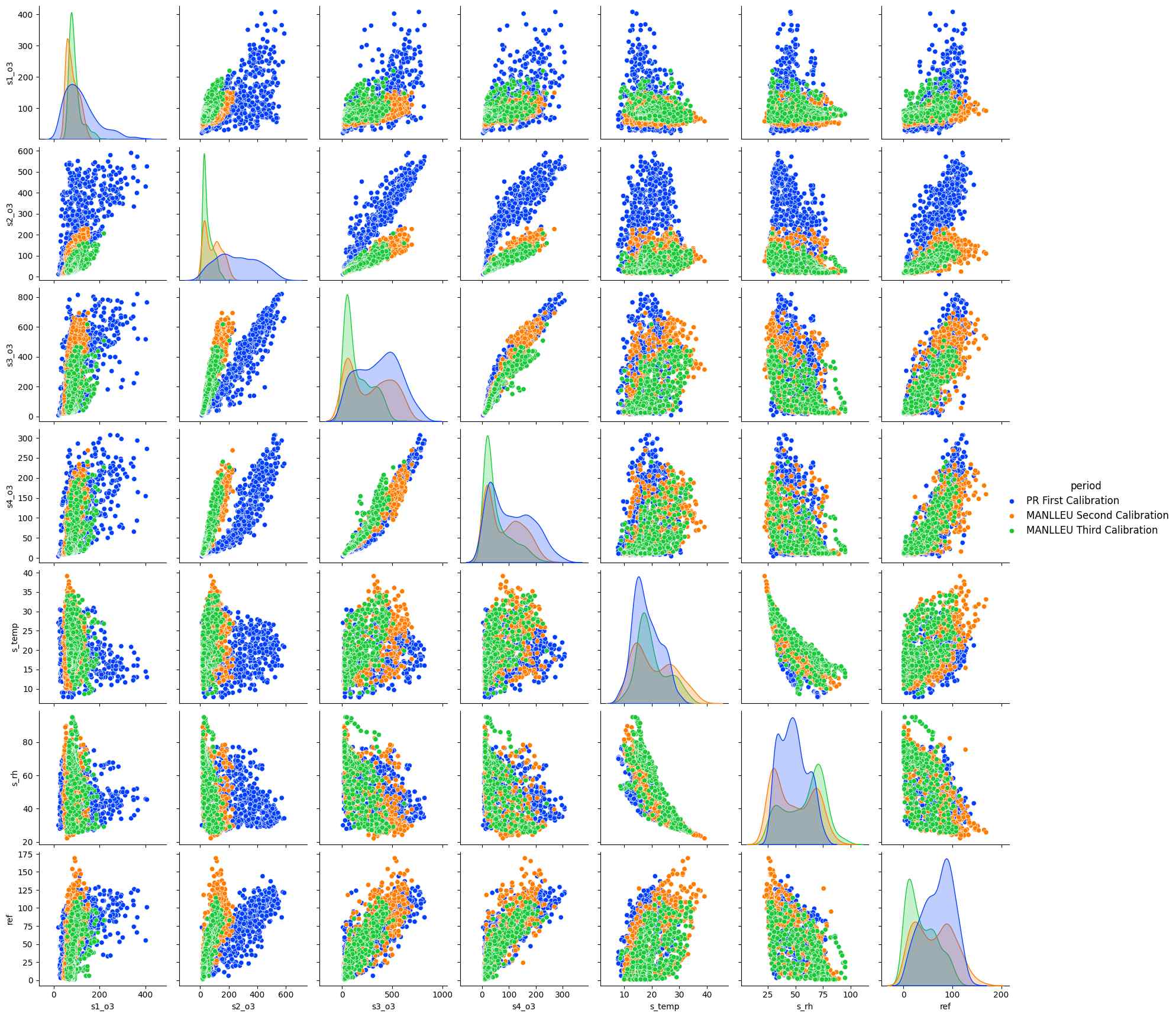
The meaning of columns:
- s1_o3 to s4_o3 are O3-specific metal oxide sensors
- s_temp is the temperature sensor
- s_rh is the relative humidity sensor
- ref is the reference data
Calibration Models
Having identified the necessities of developing a sensor fusion calibration strategy, we will perform calibration studies on the sensor signals with a changing number of sensors to confirm the effectiveness of this approach. Several calibration algorithms will be employed, and we will start with multiple linear regression (MLR) to establish the baseline.
Multiple Linear Regression
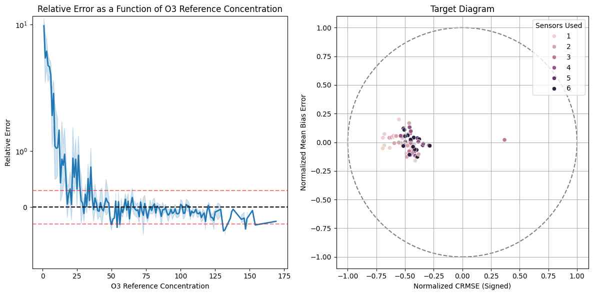
The MLR calibration is done separately on each sensor node and during each calibration period in order to compare intra-node variability and calibration effectiveness in different environments. The results and errors are summarized into data frames, and typical results are shown below.
From the relative error plot on the left, we find that most of the error is concentrated at low O3 concentration due to the sparse samples in this concentration range. The red dashed line indicates the data quality objective (DQO) defined by the European Air Quality Directive, which is 30% relative error in O3 concentration calibration. Therefore, the sensor node can only provide signals with high enough quality when the O3 concentration is above ~40 nmol/mol.
In the target diagram, a summary diagram widely used in model calibration evaluation, we have the centered/unbiased root mean squared error (CRMSE) characterizing the variability of RMSE as the x-axis, and mean bias error quantifying the average bias between model prediction and reference values as the y-axis. The distance between the origin and data points represents the RMSE. Both axes are normalized by the standard deviation of reference data in this plot. According to the plotting rules, a negative sign on the x-axis means that the standard deviation of the model is smaller than the standard deviation of reference data.
From the target diagram, we see that by incorporating an increasing number of sensors in the calibration, the calibration models exhibit a shrinking bias and CRMSE approaching the origin, meaning higher calibration quality.
In the following, Lasso regression, support vector regression, and random forest regressor will be used for calibration. The individual target diagram and relative error will be omitted and saved for the final model comparison.
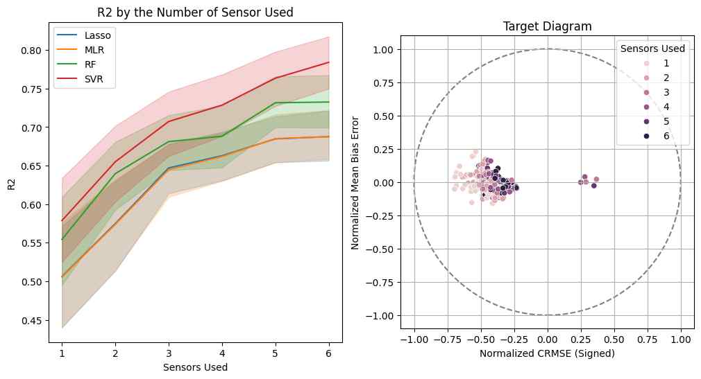
Effect of Sensor Used in Calibration
After completing all the model fitting, we need to verify the effect of the sensor fusion strategy. The R2 score of all the models done with different numbers of sensors used indicates that despite the intra-node variations, the calibration performance consistently improves with the increasing number of sensors used. Specifically, the Support Vector Regression (SVR) method provides the best calibration performance with an R2 score of 0.8. This result is consistent with the analysis done in an associated paper.
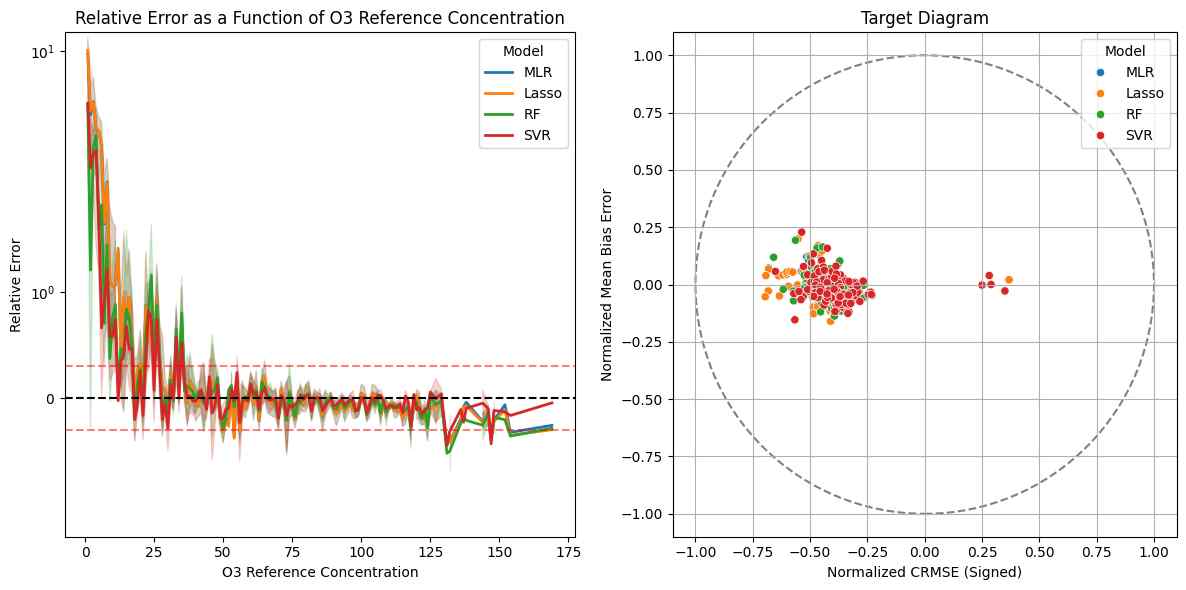
Effects of Calibration Model
As mentioned earlier, the comparison shows that SVR performs the best in terms of calibration performance. This observation has been confirmed by the relative error, all models perform well at intermediate O3 concentrations. However, SVR stands out by effectively reducing error at low O3 concentrations where sample representation is sparse. Additionally, it also reduces error at high concentrations, making calibrations that were marginally acceptable now fall within an acceptable range.
When it comes to the target diagram, where SVR produces predictions with a smaller spread in bias and a smaller CRMSE.
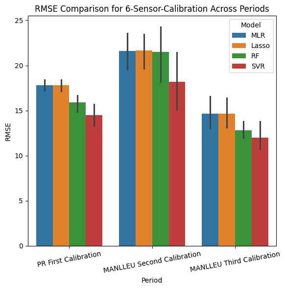
Effects of Calibration Periods
Here we compare the root mean squared error (RMSE) generated by each model in different calibration periods. We observed that the second calibration period was difficult as significant drift occurred at this stage, which was consistent with the abnormal sensor behavior identified during EDA. However, the support vector regression (SVR) model consistently performed better than all other models.
It is worth noting that Lasso regression, a regularized version of multiple linear regression that promotes feature sparsity, performed similarly to multiple linear regression. This is in contrast to another multi-sensor calibration study that I conducted recently. The discrepancy in model performance may have arisen due to two factors:
- Firstly, the limited number of sensors in each sensor node did not provide sufficient features for the model to choose from.
- Secondly, all O3 sensors were highly correlated, making it difficult for the Lasso algorithm to choose the most representative one. As a result, it either chose all O3 sensors indiscriminately or none at all, leading to the mediocre performance observed in this analysis.
Therefore, it may be more appropriate to use other more versatile linear models such as Elastic net, which is more resistant to correlated features, instead of Lasso regression.
Conclusions
From the analysis performed above, we conclude that to improve the calibration quality of regression models, consider the following:
- Incorporate sensor fusion strategy to reduce bias and prediction variability, ensuring high-quality calibration.
- Use Support Vector Regression (SVR) calibration models for the best performance, with high R2 scores, low RMSE, low bias, and low prediction variability.
- Consider sensor drift in low-cost sensors as it can significantly impact calibration quality, making sensor-fusion strategy effective in ensuring sensor node robustness and reproducibility.
Further work can be done on:
- Perform a more comprehensive analysis to provide complementary evidence for the observations mentioned above.
- Experiment with alternative machine learning models to find the best regression model for calibration tasks.
By incorporating sensor fusion strategies and SVR calibration models in sensor nodes, we can ensure accurate and reliable data, leading to high-quality calibration.