Optimizing Air Quality Monitoring: Sensor-Fusion Techniques for Precise Multisensor Calibration

This analysis compares different sensor-fusion techniques to achieve multisensor array calibration for precise air quality monitoring. Techniques used here include linear regression, neural networks, and tree-based methods.

Analysis Goal

Urban air quality monitoring requires a dense monitoring network to effectively map out the air quality distribution across regions. However, due to the inherent high cost of certified analyzers, the density of monitoring stations has been low. Low-cost sensors have been proposed to be the solution to this challenge as they are cheap to deploy and they can be calibrated by a certified analyzer for a short time, and then operate in the field for a long time.

This dataset encompasses readings from a metal oxide multisensor array, commercial temperature and humidity sensors, alongside ground truth measurements of pollutants: CO, NMHC, C6H6, NOx, and NO2. Our aim is to identify a regression algorithm that calibrates sensor array signals to precisely predict pollutant concentrations, optimizing for minimal training time and prolonged stable operation.

In this analysis, we commence with data cleaning and exploratory data analysis (EDA), followed by simple linear regression to set a baseline. Subsequently, we explore neural networks (as discussed in the original paper) and random forest to ascertain the optimal complexity for this task. Interestingly, linear regression emerged as the most effective, closely followed by tree-based methods, with neural networks trailing.

The full analysis with code can be found in this Kaggle notebook.

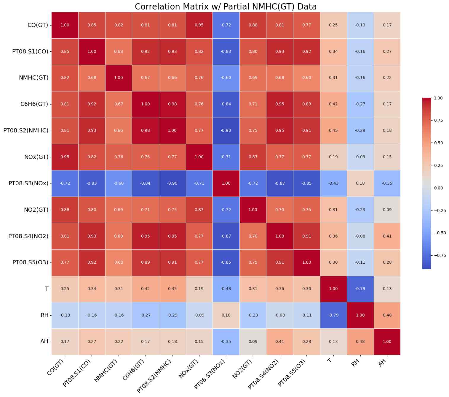
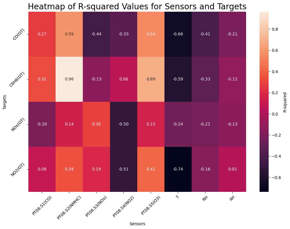
Correlation Matrix

The correlation matrix highlights correlations among four out of five metal oxide sensors, affirming their cross-sensitivity. These sensors are strong indicators of air quality-related gases, and their sensitivities are not interfered by temperature and humidity variations.

One thing stands out in this matrix is the strong correlation between benzene (C6H6) and sensor ‘PT08.S2(NMHC)’ with a correlation coefficient of 0.98, making it an easy target for us to go after first.

A correlation matrix excluding 'NMHC(GT)' data due to the broken reading.

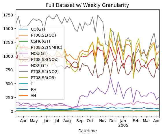
EDA

Weekly averaged data reaffirms matrix observations:

• Four out of five sensors show correlation with NOx and NO2 target analytes.
• ‘PT08.S3(NOx)’ exhibits a negative correlation with all other sensors and target analytes.

However, the correlation matrix does not capture the sensors’ continuously shifting baseline, particularly ‘PT08.S4(NO2)’. Additionally, the abrupt NO2 readout increase post-August complicates effective calibration, as will be demonstrated in later sections.

The entire time series of all sensors reading as well as analyzer ground truth.

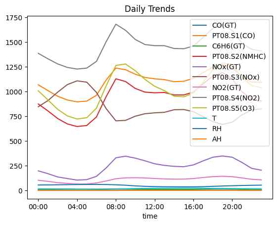
Daily Trends

NOx and NO2 levels peak at the start and end of a typical workday. The sensor array effectively captures these fluctuations.

A daily average of all time series.

Sensor Calibration

Initially, we apply linear regression using each sensor against all target analytes, training on the dataset’s first ten days (~3% of the total dataset) and validating on the remainder. Remarkably, the ‘PT08.S2(NMHC)’ sensor closely aligns with benzene concentrations, achieving an R-square of 0.96.

A heatmap of R-square from all sensors fitted to all target analytes.

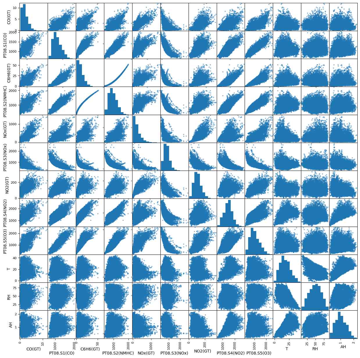
Scatter Matrix

The scatter matrix reveals that the strong correlation between ‘C6H6’ and ‘PT08.S2(NMHC)’ is unique, with other correlations displaying varying degrees of scatter.

A scatter matrix between all features.

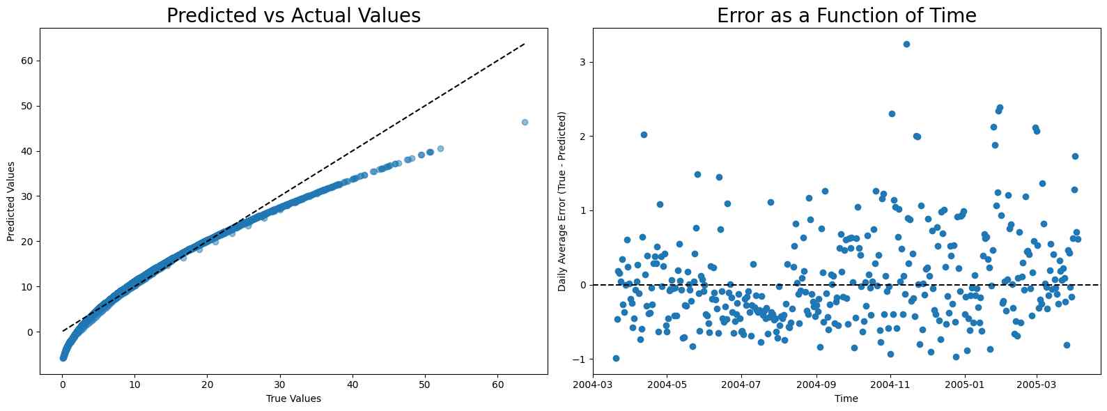
Linear Regression on ‘C6H6’ and ‘PT08.S2(NMHC)’

A detailed examination of linear regression results highlights classical underfitting due to the model’s limited flexibility. This suggests the potential for a higher-order fit.

The fitting result of C6H6 using first-order linear regression.

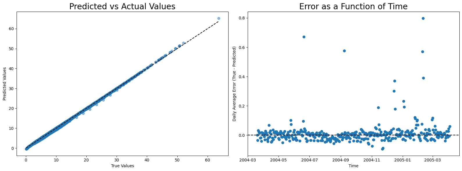
Polynomial Regression

Given linear regression’s inadequacy for benzene readouts, a quadratic function provides a near-perfect fit. A simple quadratic regression, with a 10-day training period, effectively calibrates the ‘PT08.S2(NMHC)’ sensor for year-long benzene level monitoring.

The fitting result of C6H6 using second-order linear regression.

Neural Network

While polynomial regression yields impressive results, the original study employed a ‘sensor fusion’ approach, which feeds all sensor data into a neural network model to provide the calibration. Replicating this approach, we observed a mean absolute error (MAE) of 0.52, significantly higher than the 0.06 achieved with polynomial regression, suggesting neural networks may not be a suitable choice given the dataset’s size and feature count.

The fitting result of C6H6 using neural network.

Random Forest

Trying moderately complex machine learning method, such as random forest, yields better performance than neural network, but is still no match compared to linear regression.

A brief summary of MAE scores:

• Linear regression: 0.06464961653145739
• Random Forest: 0.2284405194727994
• Neural network: 0.4388882121784993

Random Forest Calibration for Benzene.

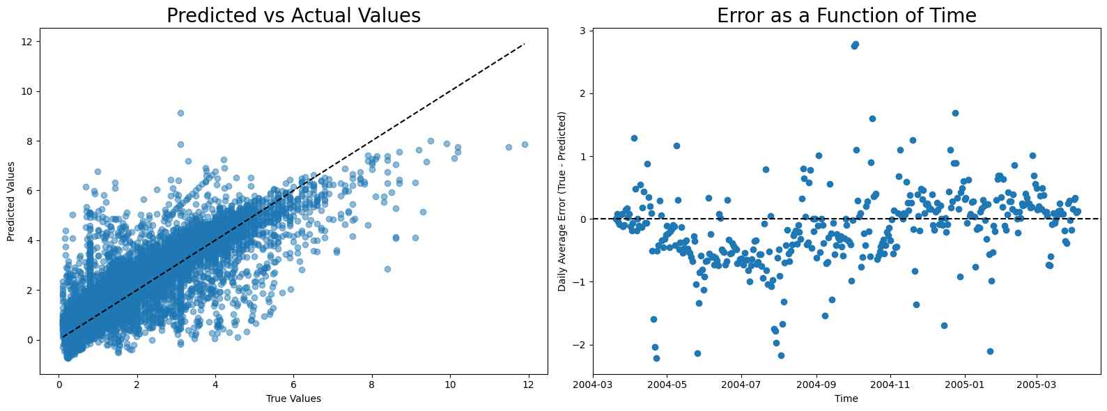
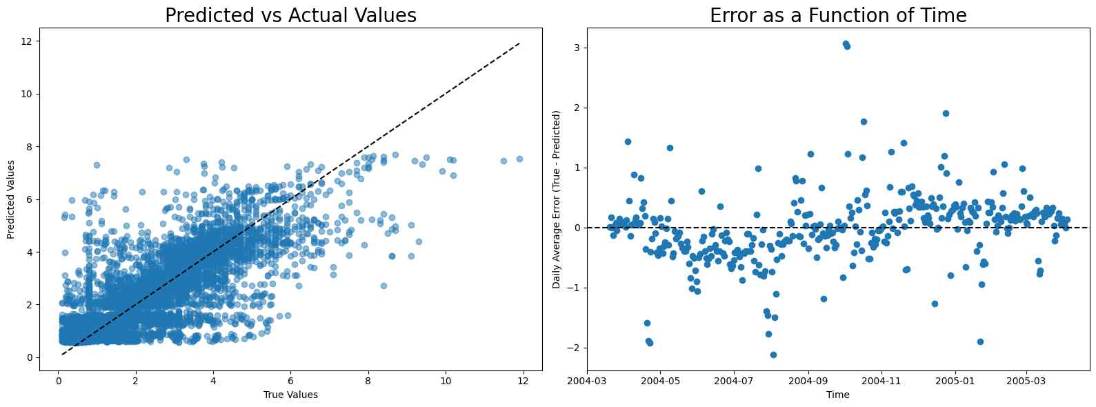
Other Pollutants

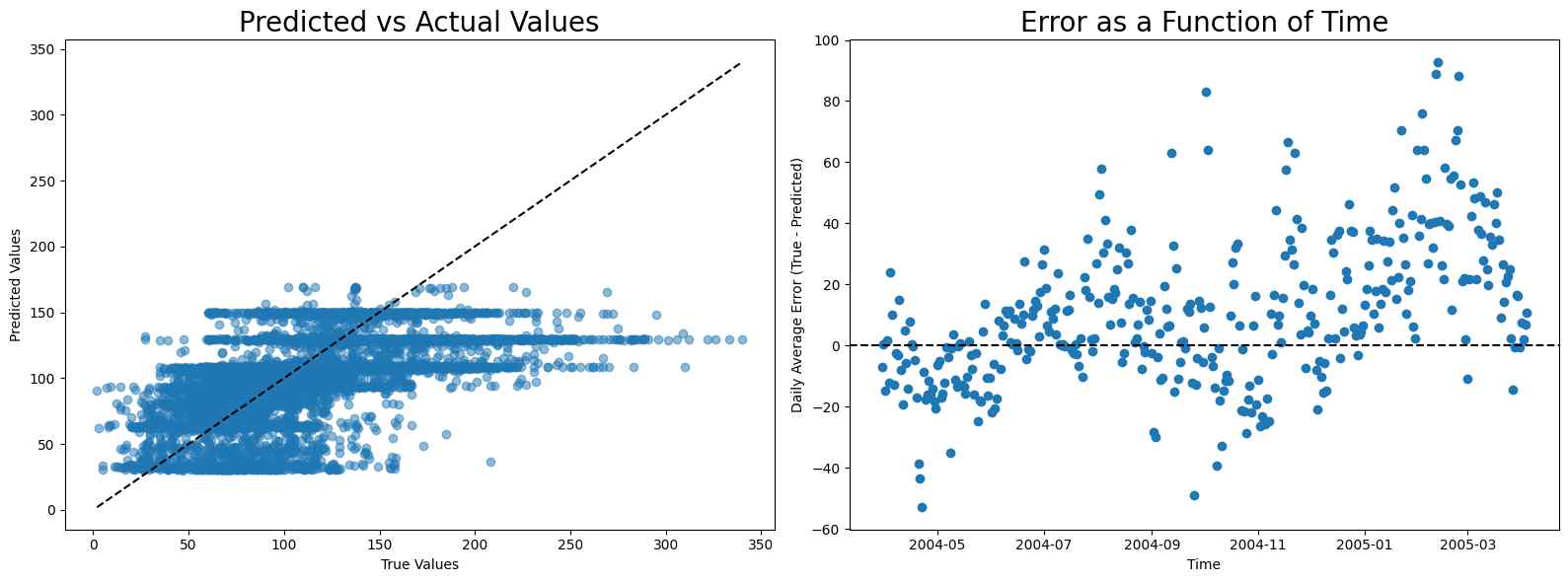
CO

Calibration for CO concentration is much more difficult. With the same training time as the neural network, the random forest provides the best performance.

MAE scores

• Linear regression: 0.631317367890475
• Random Forest: 0.5451608378533798
• Neural network: 1.021655128654683

Linear regression calibration for CO.

Random forest calibration for CO.

Neural network calibration for CO.

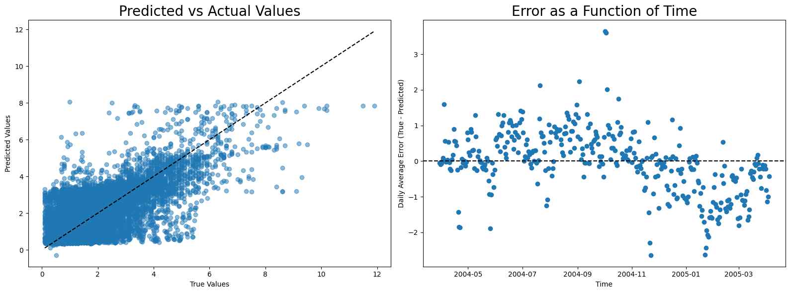
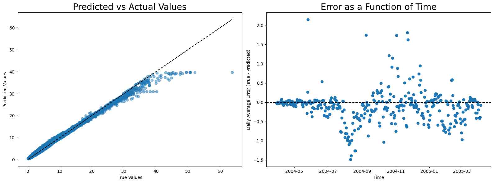
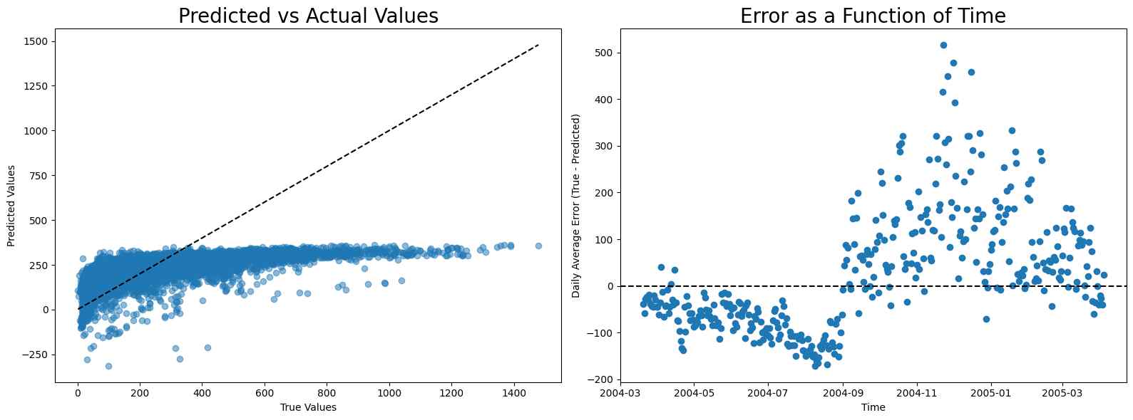
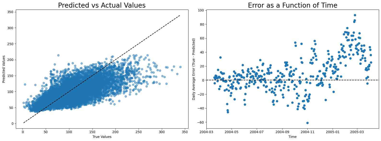
NOx

The calibration for NOx is even more difficult because of the sudden rise in NOx level after August. Notice that although linear regression has the best score, it has high error before and after August, while random forest and neural network have low error before August and high error after it, making them more appropriate compared to linear regression.

MAE scores

• Linear regression: 117.53067210253921
• Random forest: 131.48320603220608
• Neural network: 173.69570071251604

Linear regression calibration on NOx.

Random forest calibration on NOx.

Neural network calibration on NOx.

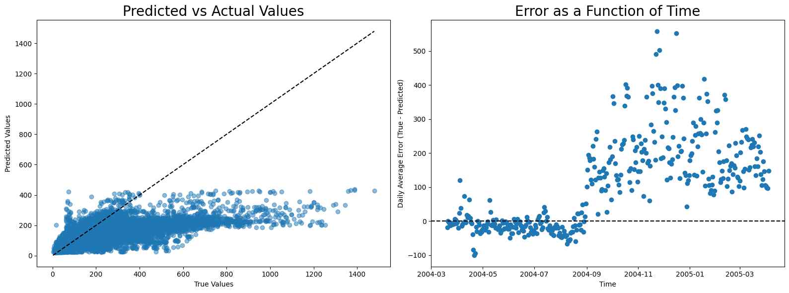
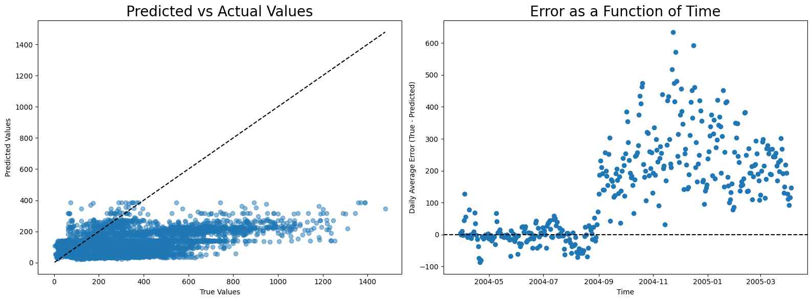
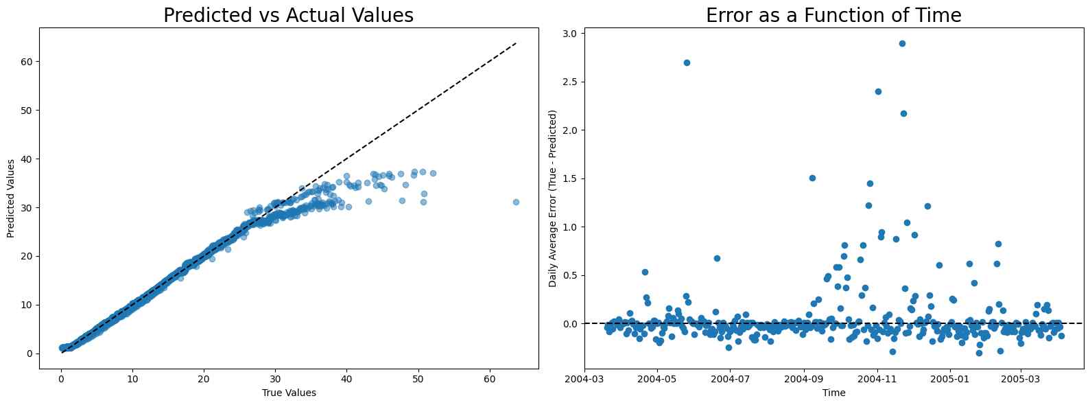
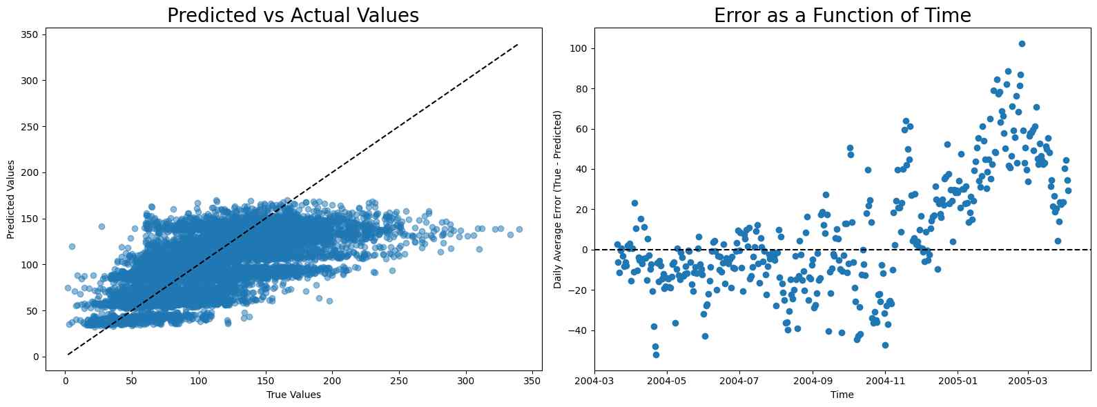
NO2

The calibration for NO2 also exhibits two periods: the first period gives reasonable fitting while the second period leads to a sudden rise in error. Here, linear regression is still the best calibration model.

MAE scores

• Linear regression: 27.22671494222509
• Random Forest: 28.167480404958546
• Neural network: 35.027760191767776

Linear regression calibration for NO2.

Random forest calibration for NO2.

Neural network calibration for NO2.

Conclusions

Developing low-cost, stable sensor arrays for air quality monitoring remains challenging. This analysis revealed that while the ‘PT08.S2(NMHC)’ sensor is notably stable and effective for benzene monitoring, the original paper’s choice of neural network for sensor fusion calibration seems suboptimal. Linear regression and tree-based methods consistently outperformed neural networks in calibration accuracy. For enhanced calibration precision, multiple linear regression with regularization or fine-tuned ensemble tree-based methods are recommended.

Thank you for reading!